Introduction
In this lesson you will learn how to use link prediction in GDS. This includes configuring and executing the pipeline as well as how to make predictions with the resulting modeling object.
GDS currently offers a binary classifier where the target is a 0-1 indicator, 0 for no link, 1 for a link. This type of link prediction works really well on an undirected graph where you are predicting one type of relationship between nodes of a single label, such as for social network and entity resolution problems.
Link Prediction Pattern in GDS
Below is an illustration of the high level link prediction pattern in GDS, going from a projected graph through various steps to finally registering a model and making predictions on your data.
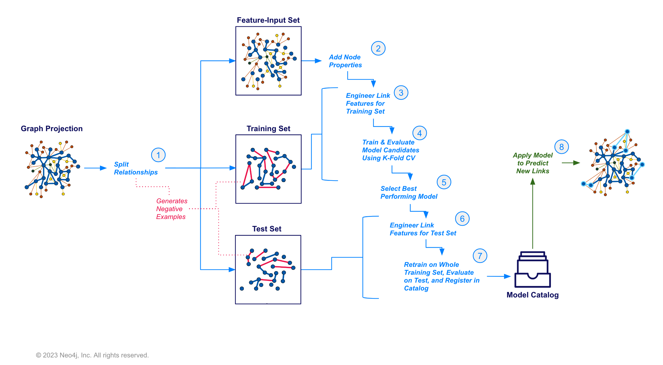
You will notice some extra steps in here that are different from node classification and other general purpose ML pipelines you may have worked with in the past. Namely, there is an additional feature-input set in the relationship splits which now comes before node property and feature generation steps. In short, this is to handle data leakage issues, whereby model features are calculated using the relationships you are trying to predict. Such a situation would allow the model to use information in the features that would normally not be available, resulting in overly optimistic performance metrics. You can read more about the data splitting methodology in our Configuring the pipeline documentation.
In addition to data leakage issues, Link prediction problems are, generally speaking, notorious for severe class imbalance and performance issues when data sampling is not approached thoughtfully. The implementation in GDS has multiple mechanisms for overcoming these issues. In summary, it boils down to sampling and weighting procedures along with choosing appropriate evaluation metrics. For further resources on this, you can see our documentation on link prediction metrics and class imbalance.
Like with node classification, the training steps will be executed automatically by the pipeline. You will just be responsible for providing configuration and hyperparameters for them.
Example: Predicting Actor Relationships with Link Prediction
Setting up the Problem
Our movie recommendations dataset, as-is, is not the best candidate for this type of link prediction since it is a k-partite graph, i.e. relationships only go between disjoint sets of nodes. In this case those sets can align with the node labels: User, Movie, Person, and Genre. For sake of showing a quick example, we will manufacture a social network out of the graph. We will filter down to just big, high grossing movies then create ACTED_WITH relationships between actors that were in the same movies together. There are a couple extra steps here to get the graph truly undirected as we need it.
//set a node label based on recent release and revenue conditions
MATCH (m:Movie)
WHERE m.year >= 1990 AND m.revenue >= 1000000
SET m:RecentBigMovie;

//native projection with reverse relationships
CALL gds.graph.project('proj',
  ['Actor','RecentBigMovie'],
  {
  	ACTED_IN:{type:'ACTED_IN'},
    HAS_ACTOR:{type:'ACTED_IN', orientation: 'REVERSE'}
  }
);

//collapse path utility for relationship aggregation - no weight property
CALL gds.beta.collapsePath.mutate('proj',{
    pathTemplates: [['ACTED_IN', 'HAS_ACTOR']],
    allowSelfLoops: false,
    mutateRelationshipType: 'ACTED_WITH'
});

//write relationships back to graph
CALL gds.graph.writeRelationship('proj', 'ACTED_WITH');

//drop duplicates
MATCH (a1:Actor)-[s:ACTED_WITH]->(a2)
WHERE id(a1) < id(a2)
DELETE s;

//clean up extra labels
MATCH (m:RecentBigMovie) REMOVE m:RecentBigMovie;

//project the graph
CALL gds.graph.drop('proj');
CALL gds.graph.project('proj', 'Actor', {ACTED_WITH:{orientation: 'UNDIRECTED'}});
This gives us a graph projection with just Actor nodes and ACTED_WITH relationships, like a 'co-acting' social network. When we use link prediction in this context, we will be training a model to predict which actors are most likely to be in the same movies together given other ACTED_WITH relationships already present in the graph. This same methodology can be used for different social network recommendation problems. For example, if instead of actors co-acting with each other we had users who were friends with each other, we could use a model like this to make friend recommendations. Likewise in fraud detection and law enforcement applications, if we have communities of suspects and victims who know or interact with each other, we could use link prediction to infer real-world relationships not already known in the graph.
Configure the Pipeline
The configuration steps are as follows. Technically they need not be configured in order, though it helps to do so to make things easy to follow.
-
Create the Pipeline
-
Add Node Properties
-
Add Link Features
-
Configure Relationship Splits
-
Add Model Candidates
To get started, create the pipeline by running the following command:
CALL gds.beta.pipeline.linkPrediction.create('pipe');This stores the pipeline in the pipeline catalog.
Next, we can add node properties, just like we did with the node classification pipeline.
For this example, let’s use fastRP node embeddings with the logic that if two actors are close to each other in the ACTED_WITH network they are more likely to also play roles in the same movies. Degree centrality is also another potentially interesting feature, i.e. more prolific actors are more likely to be in the same movies with other actors.
CALL gds.beta.pipeline.linkPrediction.addNodeProperty('pipe', 'fastRP', {
    mutateProperty: 'embedding',
    embeddingDimension: 128,
    randomSeed: 7474
}) YIELD nodePropertySteps;

CALL gds.beta.pipeline.linkPrediction.addNodeProperty('pipe', 'degree', {
    mutateProperty: 'degree'
}) YIELD nodePropertySteps;
Next we will add link features. This step configures a symmetric function that takes the properties from the node pair and computes features for the link prediction model. The types of link feature functions you can use are covered in the link prediction pipelines documentation here. For this problem we use cosine distance and L2 for the FastRP embeddings, which are good measure of similarity/distance and hadamard for the degree centrality which are a good measure of total magnitude between the 2 nodes.
CALL gds.beta.pipeline.linkPrediction.addFeature('pipe', 'l2', {
  nodeProperties: ['embedding']
}) YIELD featureSteps;

CALL gds.beta.pipeline.linkPrediction.addFeature('pipe', 'cosine', {
  nodeProperties: ['embedding']
}) YIELD featureSteps;

CALL gds.beta.pipeline.linkPrediction.addFeature('pipe', 'hadamard', {
  nodeProperties: ['degree']
}) YIELD featureSteps;
After that we configure the relationship splitting which sets the train/test/feature set proportions, the negative sampling ratio, and the number of validations folds used in cross-validation. For our example, we will split the relationship into 20% test, 40% train, and 40% feature-input. This gives us a good balance between all the sets. We will also use 2.0 for the negative sampling ratio, giving us a sizable negative example for demonstration that won’t take too long to estimate. In the context of link prediction, a negative example is any node pair without a link between it. These are randomly sampled in the relationship splitting step. You can read more on different strategies for setting the negative sample ratio in the Link Prediction Pipelines documentation.
CALL gds.beta.pipeline.linkPrediction.configureSplit('pipe', {
    testFraction: 0.2,
    trainFraction: 0.5,
    negativeSamplingRatio: 2.0
}) YIELD splitConfig;
Just like with node classification, the final step to pipeline configuration is creating model candidates. The pipeline is capable of running multiple models with different training methods and hyperparameter configurations. The best performing model will be selected after the training step completes.
To demonstrate, we will just add a few different logistic regressions here with different penalty hyperparameters. GDS also has a random forest model and there are more hyperparameters for each that we could adjust, see the docs for more details.
CALL gds.beta.pipeline.linkPrediction.addLogisticRegression('pipe', {
    penalty: 0.001,
    patience: 2
}) YIELD parameterSpace;

CALL gds.beta.pipeline.linkPrediction.addLogisticRegression('pipe', {
    penalty: 1.0,
    patience: 2
}) YIELD parameterSpace;
Train the Pipeline
The following command will train the pipeline. This process will:
-
Apply node and relationship filters
-
Execute the above pipeline configuration steps
-
Train with cross-validation for all the candidate models
-
Select the best candidate according to the average precision-recall, a.k.a. AUCPR.
-
Retrain the winning model on the entire training set and do a final evaluation on the test with AUCPR
-
Register the winning model in the model catalog
CALL gds.beta.pipeline.linkPrediction.train('proj', {
    pipeline: 'pipe',
    modelName: 'lp-pipeline-model',
    targetRelationshipType: 'ACTED_WITH',
    randomSeed: 7474 //usually a good idea to set a random seed for reproducibility.
}) YIELD modelInfo
RETURN
modelInfo.bestParameters AS winningModel,
modelInfo.metrics.AUCPR.train.avg AS avgTrainScore,
modelInfo.metrics.AUCPR.outerTrain AS outerTrainScore,
modelInfo.metrics.AUCPR.test AS testScore
Prediction with the Model
Once the pipeline is trained we can use it to predict new links in the graph. The pipeline can be re-applied to data with the same schema. Below we show a streaming example, but this also has a mutate mode which can then be used
CALL gds.beta.pipeline.linkPrediction.predict.stream('proj', {
  modelName: 'lp-pipeline-model',
  sampleRate:0.1,
  topK:1,
  randomSeed: 7474,
  concurrency: 1
})
 YIELD node1, node2, probability
 RETURN gds.util.asNode(node1).name AS actor1, gds.util.asNode(node2).name AS actor2, probability
 ORDER BY probability DESC, actor1
This operation supports a mutate execution mode to save the predicted links in the graph projection. If you want to write back to the database you can use the mutate mode followed by the gds.graph.writeRelationship command covered in the graph catalog documentation.
This predict operation also has various sampling parameters that can be leveraged to more efficiently evaluate the large number of possible node pairs. The procedure will only select node pairs that do not currently have a link between them. You can read more about the procedure and parameters for sampling in the link prediction pipelines documentation here.
Check your understanding
1. Machine Learning Steps
Which step in the link prediction pipeline adds link features from node properties?
-
❏
addLinkFeature -
❏
combineNodeProperties -
❏
addNodeProperty -
✓
addFeature
Hint
A link feature could be considered a feature.
Solution
The answer is addFeature.
You can read more about adding link prediction features in the GDS documentation.
2. Pipeline Configuration
What are the 3 relationship sets created by the configureSplit step in the link prediction pipeline?
-
❏ train, validation, and test
-
❏ train, test, and hold-out
-
✓ train, test, and feature-input
-
❏ validation, test, and hold-out
Hint
These are the key elements of a Neo4j property graph.
Solution
The answer is train, test, and feature-input.
You can read more about configuring relationship splits in the GDS documentation.
Summary
In this lesson you learned about the different steps in the link prediction pipeline and how to run the pipeline in GDS.