
Gatekeeping
In the previous lesson Closeness and Harmonic iFull definition for centrality (opens in a new tab)How important a node is within a graph. Each centrality algorithm defines importance differently. scored every person by how many steps the rest of the network takes to reach them.
Algorithms in the Gatekeeping family score a iFull definition for node (opens in a new tab)A vertex in a graph. In a property graph it can carry labels and properties. by how much control they have over informational flow in the graph.
In the iGo to glossary for graph data science (opens in a new tab)Analysing data through the structure of its connections. Also the name of the Neo4j library that implements it. library, iFull definition for betweenness centrality (opens in a new tab)A score for each node equal to how often it lies on the shortest paths between other nodes. is the only algorithm in this family.
In this lesson, you'll:
- Run Betweenness Centrality on the
directediFull definition for projection (opens in a new tab)An in-memory copy of part of your database that graph algorithms run against. You choose which nodes and relationships it holds. - Rank nodes by the score it writes
- Compare two users' scores from the network
By the end of this lesson, you will understand when and how to analyze a graph for information-flow.
What Betweenness Centrality does
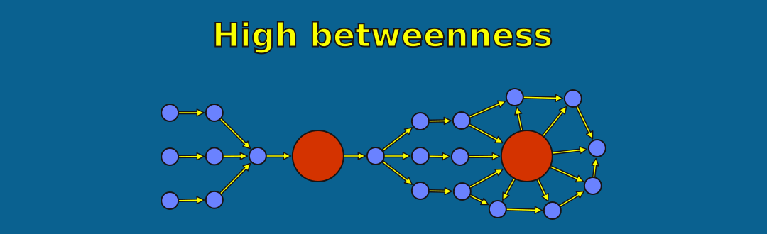
Betweenness Centrality scores a node by the shortest paths running through it.
The graph below reuses the two triangles from the Articulation lesson.
Alice and Dmitri sit on every shortest path between the two triangles.
For example, Mehmet, Mark and Dmitri cannot reach Cesar or Bridget unless they travel through Alice. Notice also, Mehmet and Mark must travel through Dmitri to reach Alice.
The same is true in reverse, from Bridget and Cesar.
We can therefore assign Alice and Dmitri with high betweenness scores — every shortest path between any two nodes must travel through Alice and Dmitri.
Gatekeepers and chokepoints
That is functionally how the algorithm works. However, you can look at it a different way.
Both Alice and Dmitri are chokepoints or gatekeepers in the network.
If Mark wants to send out a message, and have it reach anyone on the Alice side, it must travel through Alice. If Alice decides not to pass it on, it won't go further than her.
A gatekeeper is not always a chokepoint
The previous explanation correctly asserts that a node can be a gatekeeper. However, it risks implying that all gatekeepers must be chokepoints. This is not true.
Imagine a graph of a Roman Emperor's familial and political circle.
In this graph, there are no chokepoints, per se. Octavia speaks to Livia and Julia directly, and reaches everyone else only by passing through Livia first.
Agrippa can get a message to Julia through Maecenas, Livia and Octavia — several hops away, and every one of them indirect.
However, the shortest path from any one node to most other nodes goes through Augustus in almost every case.
Augustus is not a chokepoint, but he is on the shortest path for almost every message sent through the graph between other nodes. In this case, he too has high betweenness.
Look again at the route query
In the Explore the graph lesson you ran this query for 170 and 178, then for 1607 and 1802. Both routes ran from nodes with single iFull definition for relationship (opens in a new tab)A named, directed connection between two nodes. Every relationship has a type, a start node and an end node. and through nodes with hundreds of relationships.
Run it again now.
MATCH path = SHORTEST 1
(:Person {id: '170'})-[:MESSAGED]-+(:Person {id: '178'}) // (1)
RETURN path- 1
One route between one named pair
Double-click the nodes in the chain to see the full scope of their relationships. Try to guess which of these nodes will have the highest betweenness.
Betweenness Centrality
Betweenness Centrality takes every pair of nodes in the graph and counts how many of the shortest routes between them pass through each node.
Run it now on the directed graph.
CALL gds.betweenness.write( // (1)
'directed', // (2)
{ writeProperty: 'betweenness' } // (3)
)
YIELD nodePropertiesWritten // (4)
RETURN nodePropertiesWritten- 1
Runs Betweenness Centrality and writes each score back to AuraDB instead of returning it
- 2
The projection to read the graph from
- 3
The property every
:Personis given, holding their score - 4
How many people were given the property
Your output should look like this:
| nodePropertiesWritten |
|---|
| 1899 |
Every (:Person) node now carries a betweenness score.
Read the property back
Run the following query to rank people by their betweenness scores.
MATCH (p:Person)
RETURN p.id AS person,
toInteger(p.betweenness) AS betweenness,
COUNT { (p)-[:MESSAGED]->(:Person) } AS messages
ORDER BY betweenness DESC
LIMIT 6Your output should look something like this:
| person | betweenness | messages |
|---|---|---|
| 32 | 161047 | 457 |
| 103 | 125511 | 739 |
| 105 | 118599 | 685 |
| 42 | 118063 | 346 |
| 400 | 110395 | 443 |
| 9 | 97318 | 1091 |
Person 32 holds the highest at 161,047, having sent 457 messages.
Person 9 sat in the middle of the first route you traced, and sent 1,091 messages. On routes that follow the direction of each message, 9 is sixth with 97,318.
Interpretation
Notice here how the betweenness score is not predicted by how many messages someone sent. Person 32 sent many fewer messages than others in this list, but still comes out on top.
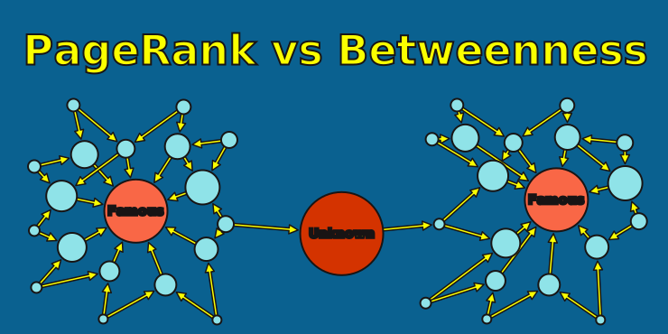
The following query returns a graph of Person 32 and Person 1624 including their local neighbourhoods. Run it now, and examine the graph.
MATCH path = (:Person {id: '32'})-[:MESSAGED]-(:Person)
RETURN path
UNION
MATCH path = (:Person {id: '1624'})-[:MESSAGED]-(:Person)
RETURN pathThe query should return a relatively large visualization of both nodes' local networks, including some shared nodes.
What the visualisation shows
Person 1624 sent 640 messages. Person 32 sent approximately one-third fewer messages overall.
Person 1624's betweenness score still sits well below Person 32's.
To see what Betweenness Centrality is seeing, take a closer look at the local graph structure of each node.
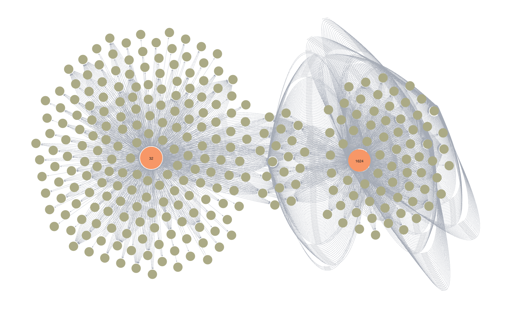
You should notice that, while Person 1624 sent more messages, their broader network is also more insular, with lots of repeat messages to the same people, and few of them leaving the locale.
Person 32 sends fewer messages, but to more people. Each new node in that network offers another chance for a shortest path between any pair to include Person 32.
What Betweenness tells you about this graph
Betweenness is useful for analyzing the low-betweenness sections of your graphs, too.
Run this to count the people at zero.
MATCH (p:Person)
RETURN sum(CASE WHEN p.betweenness = 0 THEN 1 ELSE 0 END) AS zero,
sum(CASE WHEN p.betweenness > 0 THEN 1 ELSE 0 END) AS nonzeroYour output should look like this:
| zero | nonzero |
|---|---|
| 670 | 1229 |
670 people sit on nobody's shortest route. 1,229 people sit on at least one.
Other considerations
As with all algorithms, the meaning of a Betweenness Centrality result will change based on the analyzed graph.
For instance, had you run it on the undirected projection, a route could also follow a message backwards. Person 9 would have risen from 97,318 to 129,080, and Person 32 would have fallen from 161,047 to 107,236.
Similarly, a graph that modelled each message as its own node would put every pair of people two steps apart, and every route between them would run through a message. In such a model, message nodes would likely take a larger share of top-band results.
Later, you will learn more about the nuances of Betweenness Centrality in its dedicated lab.
Check your understanding
Sign in to test your knowledge with interactive questions, track your progress, and earn a certificate when you complete the course.
Sign in or register